Applying Statistics Knowledge to Calculators
This document is for students who learned Statistics on Excel but also require calculator expertise. For example, if you intend to take the CGA (accountants) examination, you need to learn how to do statistics on calculators. You can add to your Excel knowledge and be adept at both calculators and Excel. If you are taking Seneca College Marketing, International Business, Finance, or the 2-year Accounting diploma then Excel is sufficient. The web site growingknowing.com includes PowerPoint Slides and Textbook that show both Excel and Manual calculations. In the Statistics Appendix of growingknowing.com there is also a "Study Formula Sheet" that compares manual and Excel formulae. In growingknowing.com, answers to practice questions are calculated to provide a range of answers where needed so both calculator or Excel solutions are graded correctly. This document provides calculator instruction with the assumption you already know the Excel method for finding statistical solutions.
Time spent learning statistics on Excel is a good investment. Calculators are not practical on datasets with millions or even hundreds of data items. Calculators do not allow easy sharing of results, formatting, auditing, or printing. CGA also recognizes computer skills are critical for business success.
The calculator recommended by Seneca is the Texas Instruments BAII Financial calculator (BAII). This calculator has many functions that are time-savers for statistics students. We strongly recommend you read the BAII instructions in "Overview of Calculator Operations", practice using the basic calculator functions and get to know the calculator. Some general functions you may use are:
- If you follow your calculator instructions, you can change the calculation method from Chn (chain) to AOS (algebraic operating system) if you want multiplication and division operations done before addition and subtraction, regardless of the order you enter them. The default is Chn and this document assumes you have the calculation method set to Chn.
- You can alter some settings temporarily and press 2nd CLR WORK to reset the defaults, but note that any data entered is also cleared. Read your calculator manual to learn more about clearing and resetting your calculator.
- Don't forget to clear memory before you begin a new calculation as described in your calculator instructions manual to prevent errors.
- There is a statistics worksheet in the BAII calculator, but you may not get full marks if you use STAT functions to derive test answers. If a professor wants to see how you derived the answers you have to do manual calculations.
We will now present calculator methods for every topic you learned on Excel. The order of topics may seem a bit strange but the idea is to provide the maximum ability and confidence in the shortest time. Reminder: this document is for students who have learned statistics using Excel so we assume you know the topics already. If you are learning statistics for the first time, this document is not for you.
Topics that are easy to do on calculators:
For more than a third of the topics we learned, the calculation is simple enough that a computer is not required. In some cases, you will be able to follow the same formula as you learned in Excel, once you substitute multiplication signs for asterisks, √ x for SQRT, and an exponent using the number following a ^. Remember to perform calculator operations in the correct order. An easy way to remember the correct order of operations, from first to last, is BEDMAS (Brackets, Exponents, Division, Multiplication, Addition, and Subtraction). For example, for 1- 1/k2, you would do the exponent operation first, then division, and lastly subtraction.
| Range | For range, we subtract the smallest number from the largest number in the dataset. We used Excel to find the largest and smallest values using =MAX and =MIN, but if your dataset is small, you can easily see the largest and smallest value. In business, with a large dataset, you would need Excel or it would be too easy to miss the smallest or largest value. |
|---|---|
| IQR | Interquartile range is a subtraction of two numbers (3rd quartile - 1st quartile). |
| Empirical Rule | You simply add the standard deviation to the mean or subtract it from the mean to find the empirical rule. |
| Coefficient of Variation | For coefficient of variation, we divide standard deviation by the mean and multiply by 100. |
| Frequency Distribution | Relative frequency is found by adding up the frequencies for the categories of interest and dividing this total by the total of frequencies for all categories. |
| Probability | For Probability questions (usually contingency tables) perform the same add, subtract, multiply and divide operations specified in Excel formulae. Just replace asterisks with multiplication signs and the formulas will work on a calculator. Remember to perform operations in the correct order using BEDMAS (Brackets, Exponents, Division, Multiplication, Addition, and Subtraction). |
| Mode | Mode is the value or item that occurs most often in a set of data. In a small dataset you can see the mode by just looking. The Excel =MODE function must be used with care because it does not display multi-modes without an awkward combination of keystrokes. |
| Mean | Everyone has calculated the mean (average) many times in high school. You add up all the numbers to get the total and divide the total by the count of all numbers you were given.
Note: On the BAII calculator, you can enter your data into a statistics worksheet. For example, given data: 1, 2, 3:
|
| Median | For median, if you have an odd number of data items, you take the middle data item in the list of sorted numbers. Excel =MEDIAN will sort the numbers for you, so remember to sort the numbers before determining the median manually. If the count of data items is even there is no single middle data item, so the median is the average of the middle two data items in the sorted list. |
| Standard Deviation | Standard deviation is the square root of the variance. If you use the Excel standard deviation function, =STDEV or =STDEVP, Excel will calculate the variance for you and then take the square root for the standard deviation. Assuming your question provides a variance, enter the variance and press the calculator button for square root √ x . If variance is not provided, only raw data, you will have to calculate variance first. Please note the symbol for standard deviation in statistics formulas is σ, called sigma. |
| Chebyshev | There is no function in Excel for Chebyshev so we use the same formula in Excel to find Chebyshev as a calculator student. Chebyshev = 1- 1/k2. The button to square a number on calculators is usually x2. Remember BEDMAS (described above) and do the exponent operation first, then division and then subtraction. |
| Binomial Mean | We find the binomial mean by multiplying two numbers (n × p). |
| Binomial Variance | The binomial variance is n × p × (1-p). Using BEDMAS, you would calculate the 1-p first since it is within brackets, and then do the multiplications. |
Topics you already know how to do on a calculator:
| Skewness | We did not use the Excel Skewness function. Instead, we used Excel like a calculator using the manual formula with multiply and divide operations. Therefore, you can use the same formula except that you will have to calculate average, median and standard deviation manually if they are not provided in the question. |
|---|---|
| Percentile | We found percentiles using the same formula as calculator students instead of using the Excel formula. The only task Excel did for you in percentile was sort data. You will need to sort your percentile data manually, but the calculation itself is the same on calculators as you learned on Excel. |
| Z Score | We did not use the Excel z score function =STANDARDIZE because the calculation is so simple. The only difference is you will have to calculate average and standard deviation manually if they are not provided in the question. |
Topics that are very different using calculators:
| Combination | We used the Excel function =COMBIN(n,r) for combinations. On a calculator, you use the nCr button. How would we find the combination if we take groups of 2 at a time out of a a group of 5 items? On the BAII calculator, press 5 2ND nCr 2 = buttons to get an answer of 10. Most calculators require you press a button called '2nd' to get access to an nCr function. |
||||||||||||||||||||||||||||||||||||||||||||||
|---|---|---|---|---|---|---|---|---|---|---|---|---|---|---|---|---|---|---|---|---|---|---|---|---|---|---|---|---|---|---|---|---|---|---|---|---|---|---|---|---|---|---|---|---|---|---|---|
| Permutation | We used the Excel function =PERMUT(n,r) for permutations. On a calculator, you use the nPr button. For example, on the BAII calculator, press 5 2ND nPr 2 = buttons to get an answer of 20. Most calculators require you press a button called '2nd' to get access to an nPr function. |
||||||||||||||||||||||||||||||||||||||||||||||
| Expected Value | In our textbook, we calculate discrete expected value by multiplying each value of x by its probability, then add up all the answers to get the expected value. In the PowerPoint slides, we showed the same method but we also included a shortcut using the Excel =SUMPRODUCT() function. On the BAII Plus calculator, you have to perform each multiplication but if you press the + button after each multiplication you will end up with the sum of all the products with no additional effort. For example, given data: 2, 3 and probabilities: 0.25, 0.1:
|
||||||||||||||||||||||||||||||||||||||||||||||
| Discrete Variance | Excel has no discrete variance function so we used Excel math functions but were able to do the calculation once for the first row, then drag the column down to apply those calculations to every row of data. On a calculator, you must repeat the process for every piece of data.
There are many steps but on the BAII calculator, you can press the + button after each iteration of step 1, accomplishing steps 1 and 2 in one combined step. For example, using the table below, you would press buttons: 0 × .65 = + 1 × .10 = + 2 × .20 = + 3 × .05 = to get expected value 0.65. Steps 3, 4 and 5 can also be done together as one step in the same manner. Don't use this short cut if your professor wants you to show each product for full marks.
We suggest you check your calculations twice because with so many steps, it is easy to enter one number incorrectly. |
||||||||||||||||||||||||||||||||||||||||||||||
| Variance | Calculating Variance with Excel is fast and easy using the =VAR function for a sample or =VARP for population data. Following are the steps to calculate Variance manually:
On the BAII calculator, you could use the following method to save time: You should practice doing variance by calculator a few times so you can do each step from memory and with confidence. Use growingknowing.com to practice questions until you can do it correctly 3 or 4 times in a row. The following table summarizes these calculations, where mean = x̄ = (1+5+3)/3 = 9/3 = 3 and xi represents each data item:
|
||||||||||||||||||||||||||||||||||||||||||||||
Topics that are difficult on a calculator:
| Binomials | In Excel we used the =BINOMDIST() function to calculate Binomial Probability. BINOMDIST includes a parameter called CUMULATIVE enabling multiple calculations that are automatically summed. On a calculator, there is no cumulative parameter. As an example, to find a binomial probability of less than 20 successes, you must calculate each probability from 0 to 19 separately, then add each result to find the cumulative probability of less than 20. This method is a lot of work, error-prone, and very slow so not appropriate when working for an actual business. The formula is intimidating at first glance. But, if you look carefully, you see the first part of the formula is a combination, so use your nCr button on the calculator to find that portion of the formula quickly. You need to know how to use different exponents on your calculator and the button for this is usually called yx. Please review the growingknowing.com website textbook for manual binomial calculation examples, however, one example is provided here for your convenience.
Binomial probability P(x) = nCxpx(1-p)(n-x) where n is the number of trials, x is the number of successes you want, and p is the probability of each trail. Example:What is the binomial probability for 3 successes if you have 6 trials and the probability for each trail is 0.25. To answer this question, n = 6, x = 3, and p = .25.Step 1: Push buttons: 6 2ND nCr 3 for the combination answer of 20. Step 2: Find px by pushing buttons: .25 yx 3 = to get 0.015625. Step 3: Find (1-p)n-x: 1-p is 1 - .25 = 0.75. Next n-x is 6 - 3 = 3. Enter .75, press yx button, press 3 to get 0.421875. Step 4: We now multiply: 20 x .015625 x .421875 = 0.131835938 The answer is 0.1318. If we want the probability of less the 3, we would need to do the same exercise for x = 0, x = 1, and x = 2 then add the results up for the answer. For the probability of more than 3, again you would do the calculations for x = 0, x = 1, and x = 2 and subtract the result from 1. For the probability of between 4 and 6 inclusive, you would do all the calculations for x = 4, x = 5, and x = 6 and add the results. Please see the textbook for more examples. You should do some practice questions and you can use the website or Excel to check your answers. Note that if you are not required to show every calculation, Step 3 could be done by pressing buttons: ( 1 - .25 ) yx ( 6 - 3 ) . |
||||||||
|---|---|---|---|---|---|---|---|---|---|
| Normal Distribution | In Excel, you were taught to do Normal Distribution questions directly from data to the probability answers. With calculators, we must first calculate z using the formula z = (x - mean) / Standard Deviation. Then use the cumulative normal table to lookup the probability. The z calculation is an interim step on calculators that cannot be skipped. Calculators allowed on the CGA test have no button for normal distribution probabilities so you must use a printed table to find z. There are small differences in how tables are displayed. Use the Cumulative normal table (Appendix E in our website) for z values. You must be careful if your book provides both a CUMULATIVE and a STANDARD normal table. Excel uses cumulative standard normal values. We have used the Cumulative table for our manual calculator examples, since the cumulative table is the easiest to understand and use. The following link will bring up the cumulative normal table in a new window that you can keep open while you continue working on this topic: Cumulative Areas Under the One-Tailed Normal Curve. We recommend you review all of the "Manual" calculations in the entire textbook topic "Normal Probability" in the growingknowing.com website. We recommend you do lots of practice questions. As with Excel, there are three types of questions; more-than, less-than, and between. Since z values are used in many statistics formulas in our course, we will review each formula below for every topic using z. |
||||||||
| Hypothesis Means and Hypothesis Proportion | The only calculation done differently on calculators in Hypothesis Means or Proportion is the Decision Rule. Excel finds the z value for a Decision Rule using the =NORM.S.INV function but calculator students must use the Cumulative Normal Table. Basic math functions are also different, for example use calculator button √ x instead of Excel's SQRT, and × for multiplication instead of *. Tip: you can always use Excel to check your calculator answers until you get used to the Manual method. |
||||||||
| Decision Rule | |||||||||
| Two-Tail Test: | Add alpha divided by two to the confidence level to find the probability just you did to find the value to place in the NORM.S.INV function of Excel. You must then scan the Cumulative Normal Table for that probability. Look for the closest value as the table has gaps so you may not find an exact match. The gaps occur because the table uses only two decimal points for z. If there were more decimal points provided, the table would not have gaps but would be too lengthy to be workable. Once you find the nearest probability in the table, read across and up for the z value. Excel and the Table Method will not give exactly the same answers as Excel because the Cumulative Table is limited to z values of 2 decimal points. For example, the two-tail test for a confidence level of 62.12% is: .6212 + (1-.6212)/ 2 = .8106. We find .8106 in the table and can scan across to find a z value of .8, and if we scan up we find an additional z value of .08 giving us a z value of .88. 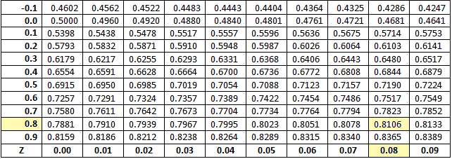 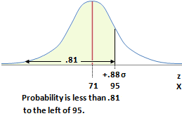 |
||||||||
| One-Tail Test: | Look up the confidence level as a probability in the Cumulative Normal Table exactly as you did for the Two-Tail test above. The only difference between one-tail and two-tail is the method to find the probability. For example, given a confidence level of 81.06%, we look for .8106 in the table. Using the table, we find a probability of .8106 has a z value = .88.
In your Excel class you learned how to state the Hypothesis question, find the Test Statistic, decide whether the Decision Rule was positive or negative, and determine whether to Reject a Hypothesis; these skills are exactly the same for calculator and Excel users. Decision Rule: Example 1Calculate the Decision Rule for a 90% confidence level using 1 and 2 tail tests, then compare the answers.1-tail Decision rule at 90% confidence = .9000 Lookup .9000 in normal table, and find z = 1.28 which is .8997. If we go to z = 1.29 we see .9015 which is not as close as .8997. Answer z = 1.28 is the best fit. 2-tail decision rule at 90% confidence = .9 + .1/2 = .9500. Lookup .9500 and we find z = 1.64 for .9495 but z = 1.65 is .9505 so each value is .0005 too small or too large. The best fit is to take the average, so z = 1.645 which is half-way between 1.64 and 1.65. Decision Rule: Example 2Find the Decision rule for a 1 and 2 tail test using a 95% confidence level.1-tail decision rule at 95% confidence = .9500 Lookup .9500 in normal table, and find z = 1.645 as the 1-tail value of 95% confidence(the same as the 2 tail value for 90% confidence above). 2-tail decision rule at 95% confidence = .95 + .05/2 = .9750. Lookup .9750 and we find z = 1.96 and this z value is an exact match in the table. |
||||||||
| Sample Size Means: |
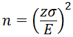
Excel does not have a function for Sample Size so Excel students use the same formula as calculator students. The only extra challenge for calculator users is to find the z value using the Cumulative Normal Table rather than using the =NORM.S.INV function in Excel. The process is exactly as the same as the 2-tail Hypothesis Decision Rule we showed above. Always use the 2-tail method when doing Sample Size calculations. The following is the formula for sample size:
Once you have the z value, you then multiply z by the standard deviation, divide by the error E, and then raise the result to the power of 2. The only step that is different for calculator versus Excel students for Sample Size calculations (mean or proportion) is calculator students use the Normal Table to find z. Example:What is the sample size required if the standard deviation (σ) is 11.55, allowable margin of sampling error is within 3.01, and confidence level is 96%?We use the 2-tail method to find z. Confidence level + alpha/2 = .96 + .04/2 = .9800. If we look up .9800 in the table, we find .98 is half way between 2.05 and 2.06 so pick 2.055 as the best fit. Now that we have z, we can now just plug it into the formula. Sample Size = n = (zσ/E)2 = (2.055 x 11.55 / 3.01)2 = 62.2. The calculation of Sample Size for Proportion is similar. You use the normal table to find the z value, and then plug the numbers given into the formula. |
||||||||
| Confidence |
There is no Excel function for Confidence proportion so Excel and calculator students use the same method once the z value is found. We use the Normal table to find the z value, the same two-tail method we used in Sample Size and the Decision Rule for Hypothesis Means. Both Excel and calculator students add the Margin of Error to the mean to find the upper confidence interval and subtract the Margin of Error for the lower confidence interval. Always use the 2-tail method when doing Confidence or Sample Size calculations. For Standard Error, Excel and calculator students use the same method because Excel has no function to calculate Standard Error. Standard Error is the standard deviation divided by the square root of n where n is the sample size. For Confidence Means, Excel has the =CONFIDENCE function to obtain the Margin of Error. For calculators, we multiply the Standard Error by the z value to obtain the Margin of Error. Again, the z value is a 2-tail method shown in Sample Size. Example:What is the Confidence Interval where sample is 75, mean = 61, standard deviation (σ) = 8.54, and confidence level of 96%?
|
||||||||
| T tests |
Samples under 30 are small and require the use of t instead of z. Excel has a =T.INV function to lookup t values while calculator students use a printed t Table. The following link will bring up the Student's t distribution table in a new window that you can keep open while you continue working on this topic: Student's t Distribution Table. Both Excel and calculator students use the concept of degrees of freedom to find t. Degrees of freedom (df) = n - 1. For Confidence questions, we use a 2-tail t table. Using the Student t table in growingknowing.com, you find t as follows: On the left side of the table you find the degrees of freedom column. On the top of the table, you locate your confidence level in the Two-Tail row, then scan down the confidence level column to read the t value that corresponds with the appropriate degrees of freedom. Once you have the t value, the calculations for small sample confidence are the same as large sample confidence except you use t instead of z. Be aware t tables can be confusing if you switch textbooks because each book labels the t table columns differently. All books use degrees of freedom to label the rows, but some tables label the columns with confidence level, some use 1 or 2 tail, and some label using alpha instead of confidence level. We avoid confusion at growingknowing.com by using all these labels so whatever book or label you prefer, our table is easy to use. If your advanced statistics course uses a different column label than the one you prefer, you can use growingknowing.com to see the equivalent label name. For example, the Keller textbook is popular for advanced statistics courses, and they label their t table using a 1-tail alpha value. So a Keller t.05 is the alpha value for a 1-tail test, and by looking at the growingknowing.com t table, you can see if you double the 1-tail alpha value, you can use the same column for a two-tail test. |
||||||||
| Small Sample Hypothesis |
For small sample hypothesis questions, the only difference is the Decision Rule that uses a t table instead of z. For hypothesis, you need to be sure you read the correct t table one-tail or two-tail column. Other than using the t table instead of an Excel function, all calculations are the same as large sample hypothesis above. |
||||||||
Summary
We have reviewed using calculators to provide a quick way to adapt. If you can pass statistics using Excel, you can pass using calculators. The steps are just as easy as Excel for many topics and many of the calculations you've done on Excel are basically the same on a calculator. In some topics the main difference is calculations are more time-consuming on a calculator since you have to do the same calculation repeatedly rather than simply dragging your mouse from one cell to adjacent cells to copy a calculation. All students, Excel or calculator, use simple arithmetic, square, square root, and exponents. You need to spend at least 30 minutes practicing using the printed tables. Happy calculating.