Statistics Study Formula Sheet
(Not permitted during exams)
| Topic | Manual Formula | Excel Formula | |||
|---|---|---|---|---|---|
| Central Tendency: | |||||
| Mean | Sample: |
Population: |
=AVERAGE(first : last) | ||
| Weighted Mean | 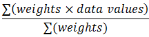 |
=SUMPRODUCT(weights, values) / n Where n = SUM(weights) |
|||
| Median | If N is odd:
|
If N is even:
|
=MEDIAN(first : last) |
||
| Mode | =MODE.SNGL(first : last) or =MODE.MULT(first : last) |
||||
| Variability: | |||||
| Range | =MAX() - MIN() |
||||
| Class Width |
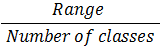
|
=range / number of classes | |||
| Variance | Sample: 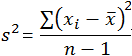
|
Population: 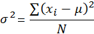 |
Sample: =VAR.S() |
Population: =VAR.P() |
|
| Standard Deviation (SD) |
Sample: |
Population: |
Sample: =STDEV.S() |
Population: =STDEV.P() |
|
| Or,=SQRT(variance) Or, =variance^0.5 |
|||||
| Skewness |
|
=3*(AVERAGE() - MEDIAN()) / SD The above formula is used in our practice questions. There is an Excel skewness formula but answers are different: =SKEW(first : last) Excel internal skewness formula is: |
|||
| Coefficient of Variation |
Sample: |
Population: |
=SD / AVERAGE() * 100 | ||
Chebyshev |
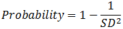 Where k = number of standard deviations |
= 1 - 1 / k^2 Where k = number of standard deviations |
|||
| Grouped Data: | |||||
| Weighted Mean |
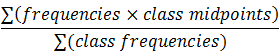 |
=SUMPRODUCT(frequencies,class midpoints)/n Where n = SUM(class frequencies) |
|||
| Median |
Class that contains middle frequency: |
class that has middle frequency: =(n+1)/2 |
|||
| Variance |
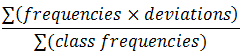 Where deviations = Population is same except divide by n, instead of n-1. |
=SUMPRODUCT(frequencies,deviations)/(n-1) Where deviations = (midpoint - mean)^2 Population is same except divide by n. |
|||
| Standard Deviation |
|
=SQRT(variance) | |||
| Position: | |||||
| Percentile | Round up if decimal; average if whole. |
= percentile / 100 * n Round up if decimal; average if whole. |
|||
| IQR | Interquartile Range = Q3 − Q1 | = Q3 - Q1 | |||
|
Upper Outlier: Q3 + 1.5(IQR) |
= Q3 + 1.5 * IQR | ||||
|
Lower Outlier: Q1 − 1.5(IQR) |
= Q1 − 1.5 * IQR | ||||
| Probability: | |||||
| P(A) P(A or B) |
same same |
||||
|
Independent: |
|||||
|
P(A and B) |
= P(A) * P(B) | ||||
|
Dependent: |
|||||
|
P(A and B) |
= P(A) * P(B|A) | ||||
|
Conditional: |
|||||
|
P(A | B) |
same | ||||
| Bayes' Rule: | |||||
|
P(A | B) |
=( P(A|B) * P(B) ) / ( P(A|B)*P(B) + P(A|Bc)*P(Bc) ) = P(B|A) * P(A) / P(B) |
||||
|
Where or = |
|||||
| Permutation | =PERMUT(n,r) Where r = number of objects selected |
||||
| Combination | 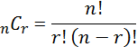 |
=COMBIN(n,r) | |||
| Discrete Distributions: | |||||
| Expected Value | =SUMPRODUCT(x,P(x)) |
||||
| Variance | =SUM(x^2 * p) - (expected value^2)) | ||||
| Standard Deviation |
=SQRT(Discrete Variance) | ||||
| Binomial Distributions: | |||||
| Mean |
|
=n*p | |||
| Variance | =n*p*(1 - p) | ||||
| Binomial Standard Deviation |
=SQRT(n*p*(1-p)) |
||||
| Probability |
|
=BINOMDIST(successes,trials,probability,cum) | |||
| Normal Distributions: | |||||
| Z Score | Sample: | Population: |
=(x - average()) / SD |
||
Or, =STANDARDIZE(x,mean,SD) |
|||||
|
Z Score is the number of standard deviations between some value of x and the mean. |
|||||
| Z to Probability | For manual calculations, look up probabilities in "Areas Under the One-Tailed Standard Normal Curve" table.
|
=NORM.S.DIST() | |||
|
Less than: =NORM.S.DIST(z score, 1) More than: =1-NORM.S.DIST(z score, 1) Between: =NORM.S.DIST(high z score,1) - NORM.S.DIST(low z score,1) |
|||||
| Probability | Excel can calculate probability directly from X, Mean and Standard Deviation, but for manual calculations, compute z score and look up probability as described above. | =NORM.DIST() | |||
|
Less than: =NORM.DIST(high value,Mean,SD,1) Where the "1" means cumulative. More than: =1-NORM.DIST(low value,Mean,SD,1) Between: =NORM.DIST(high value,Mean,SD,1) - NORM.DIST(low value,Mean,SD,1) |
|||||
| Probability to Z | Adjust probability (add or subtract .5). | ||||
| Then look up the z closest to adjusted probability. |
=NORM.S.INV(Probability) | ||||
| Probability to X | =NORM.INV(Probability,Mean,SD) |
||||
| Sampling from Normal Distribution, Mean (Central Limit Theorem): | |||||
| Standard Error |
|
Standard Error: =SD / SQRT(n) |
|||
| Probability |

|
Less than: =NORM.DIST(X,Mean,SD/SQRT(n),1) Where 1 means cumulative. More than: =1-NORM.DIST(X,Mean,SD/SQRT(n), 1) Between: =NORM.DIST(high X,Mean,SD/SQRT(n),1) - NORM.DIST(low X,Mean,SD/SQRT(n),1) |
|||
| Sampling from Normal Distribution, Proportion: | |||||
| Validation |
If Where p = population proportion |
If n*p ≥ 5 and n*(1-p) ≥ 5 use: Where p = population proportion |
|||
| Standard Error |
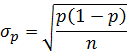
|
σp = SQRT(p*(1 - p) / n) |
|||
| Z score |
|
z = (ps - p) / σp |
|||
| Probability |
Look up probabilities in "Areas Under the One-Tailed Standard Normal Curve" table. |
Less than: NORM.S.DIST(z,1) More than: 1-NORM.S.DIST(z,1) Between: =NORM.S.DIST(high z) - NORM.S.DIST(low z) |
|||
| Confidence Intervals, Mean: | |||||
| Alpha |
|
Alpha = 1 - Confidence Level | |||
| Margin of Error |
|
=CONFIDENCE.NORM(alpha,SD,n) | |||
| Margin of Error |
|
=CONFIDENCE.T(alpha,SD,n) (small sample) | |||
| Interval |
|
= (mean - E) to (mean + E) | |||
| Confidence Intervals, Proportion: | |||||
| z |
Adjust probability (add or subtract .5) then look up z closest to adjusted probability. |
=NORM.S.INV(confidence level + alpha/2) | |||
| Margin of Error |
|
=z * SQRT(p * (1-p)/n) | |||
| Interval |
|
=(proportion - E) to =(prop + E) | |||
| Sample Size, Mean: | |||||
|
|
=NORM.S.INV(confidence+Alpha/2) Or: =(z * SD / E)^2 |
||||
| Sample Size, Proportion: | |||||
| Validation: |
|
n*p ≥ 5 and n*(1-p) ≥ 5 p*(1 − p) * (z / E)^2 |
|||
| Hypothesis Tests: | |||||
| Standard error: | Test tatistic: | ||||
| Mean |  |
1-tail: = NORM.S.INV(Confidence Level) 2-tail: = NORM.S.INV(Confidence Level + Alpha/2) Test Statistic: =(sample mean - mean) / (SD/SQRT(n)) |
|||
| Proportion | 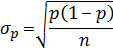 |
 |
1-tail: =NORM.S.INV(Confidence Level) 2-tail: = NORM.S.INV(Confidence Level + Alpha/2) Test Statistic: =(ps - p) / SQRT(p*(1 - p) / n) |
||
| Small Sample |  |
1-tail: =T.INV(Alpha,df) 2-tail: =T.INV.2T(Alpha,df) Where df = degrees of freedom = n - 1 |
|||
| P-Value | |
1-tail: z =NORM.DIST(sample mean, population mean, SD/SQRT(n),1) 2-tail: z = NORM.DIST(sample mean, population mean, SD/SQRT(n),1) * 2 |
|||
| Regression Analysis: | |||||
| Coefficient of Correlation: |
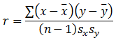 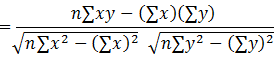
|
In Excel statistics analysis: "Multiple R" |
|||
| Coefficient of Determination: |
|
"R Square" | |||
| Regression Equation: |
|
||||
| Slope: |
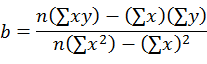 |
"X Variable" in Regression Statistics, or the heading you enter if you check "Labels" when you type data into Excel. | |||
| Y Intercept: |
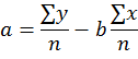 |
"Intercept" | |||
| Standard Error |
Se 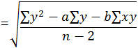 |
"Standard Error" | |||
| GrowingKnowing.com © 2010. All rights reserved. | |||||
Formula Comparisons (for population data)
| Univariate | Discrete | Binomial | |
|---|---|---|---|
| Mean | |
|
|
| Variance | |
|
|
| Standard Deviation | 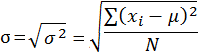 |
|
|